For high-performance computing and machine learning research, efficiently handling computations over large datasets is critical.
Last Modified: February 1st, 2023 | Reading Time: 10 minutes
Navigating the use and application of vmap may pose a challenge, particularly when modifying a function to support batch computations along a designated axis. This situation frequently emerges in machine learning, where models process batches of data iteratively for updates. Vmap, by parallelizing computations efficiently, hastens batch processing and boosts performance in instances where batch processing is crucial.
vmap acts as a crucial instrument in machine learning and related fields, enabling smooth iteration over data batches and capitalizing on hardware-accelerated vectorization for improved performance. While it might add a layer of complexity, the acceleration and efficiency it provides make vmap an essential element in executing batch computations.
To get started, let’s first create a specific function to demonstrate the concept. Here’s the function we’re going to use:
import jax.numpy as jnp


def custom_dot(x, y):
    return jnp.dot(x, y) ** 2
The function takes two input vectors, x and y, and calculates their dot product, also known as the inner product. After computing the dot product, it then squares this result to provide the final output.
We’re going to give our custom_dot function an upgrade for better versatility. Our goal? Modify it to handle batch operations, enabling us to process any number of vector pairs. One key point to remember is that each argument pair needs to have equal length to ensure proper function. For each matched pair of vectors, our function will crunch out the dot product, square it, and slot that value into the appropriate position within the output.
x = jnp.asarray([
    [2, 2, 2],
    [3, 3, 3]
])

y = jnp.asarray([
    [4, 4, 4],
    [5, 5, 5]
])

custom_dot(x, y)


>>>
TypeError: Incompatible shapes for dot: got (2, 3) and (2, 3).
When attempting to execute our custom_dot function with a list of vectors (or matrices), an issue arises due to incompatible shapes during the dot product calculation. The problem stems from the jnp.dot function, which tries to perform matrix multiplication using input shapes of (2, 3) and (2, 3). Since matrix multiplication with these shapes is undefined, an error occurs. It’s important to be cautious here because providing shapes like [a, b] and [b, c] to the custom_dot function will inadvertently trigger matrix multiplication, which is not the intended behavior. Properly interpreting the axis over the input that we wish to transform becomes crucial in order to achieve the desired outcome.
We can modify our custom_dot function to handle batches by incorporating a simple for loop.
def naive_custom_dot(x_batched, y_batched):
    return jnp.stack([
        custom_dot(v1, v2)
        for v1, v2 in zip(x_batched, y_batched)
    ])


x = jnp.asarray([
    [2, 2, 2],
    [3, 3, 3]
])

y = jnp.asarray([
    [4, 4, 4],
    [5, 5, 5]
])


naive_custom_dot(x, y)

>>>
Array([ 576, 2025], dtype=int32)
The naive_custom_dot function iterates over each pair of vectors from the input arrays x and y. It uses the zip function to create pairs of vectors. For every pair, it applies the custom_dot function to compute the squared dot product. The result is a vector, where each element corresponds to the squared dot product of the respective pair of input vectors. For instance, the first element of the output vector corresponds to the operation performed on the first pair of vectors, the second element pertains to the second pair, and so on. This allows us to handle batches of vector pairs, although it does so in a less efficient manner.
You don’t always have to use vmap, but if you aim to extend a function to support batch operations, we highly recommend it. Using vmap brings several benefits. It improves code readability, enhances code reusability, and ultimately, boosts performance. Lets look how vmap looks like actually,
# The remaining arguments in vmap are intentionally omitted in this post because they are not necessary for the purpose of the current discussion
jax.vmap(fun, in_axes=0, out_axes=0, ....)
Now, let’s apply vmap to the custom_dot function to enable batch processing, as we described in the previous section.
batched_custom_dot = jax.vmap(custom_dot, in_axes=[0, 0])


x = jnp.asarray([
    [2, 2, 2],
    [3, 3, 3]
])

y = jnp.asarray([
    [4, 4, 4],
    [5, 5, 5]
])

batched_custom_dot(x, y)

>>>
Array([ 576, 2025], dtype=int32)
Let’s break down this example and see what’s happening in the following steps:
In reality, in_axes holds no hidden secrets. It processes parameters from the list or tuple, facilitating batch operations as described. By providing essential information on how to handle arguments, in_axes actively empowers batch processing.

In our specific case, the in_params argument for vmap is set as [0, 0], which provides instructions on how to handle the batch axis for each argument. In this configuration:
Often, we interpret integers as referring to elements in 1-D arrays and rows in 2-D arrays. That is, an in_axes value of 0 for a 2-D array would indicate that each row is a separate batch item. However, as we move to higher dimensions (3-D arrays and beyond, also known as tensors), this straightforward interpretation of the axes as rows and columns doesn’t hold. Instead, we refer to each dimension by an integer representing its axis. In a 3-D array, for example, we have axes 0, 1, and 2, each representing a different dimension in the data. The semantics of each axis—what it “means” in the context of your data—will depend on the specifics of the data and the operations you are performing.
Before we proceed to the next example, let’s take a moment to delve deeper into the potential values that can populate the in_axes parameter. Building this understanding will strengthen our intuition about how in_axes influences the behavior of vmap and what its use is. Lets say that we have some function which takes two arguments which we name it as X and Y:
The animations shown in Figures 4, 4a and 4b encapsulate the cases we’ve discussed above, demonstrating how vmap operates with different in_axes configurations. However, remember that you can use different combinations of values in in_axes, including the use of None. Whether these combinations make sense largely depends on the shapes of the function’s inputs, the operations performed on these inputs, and the desired output.
Now, let’s shift our focus from the custom_dot function and delve into the JAX vmap documentation. Here, we’ll find an example that showcases the usage of the vmap function to extend a vector dot product to a matrix-matrix product. In the upcoming sections, we will explore this example to deepen our understanding of vmap’s functionality across all three defined functions
import jax.numpy as jnp

vv = lambda x, y: jnp.dot(x, y)  #  ([a], [a]) -> []
mv = vmap(vv, (0, None), 0)      #  ([b,a], [a]) -> [b]      (b is the mapped axis)
mm = vmap(mv, (None, 1), 1)      #  ([b,a], [a,c]) -> [b,c]  (c is the mapped axis)
Let’s examine this example graphically to better understand how the commented results are achieved and the rules when using vmap for different situations.
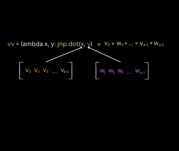
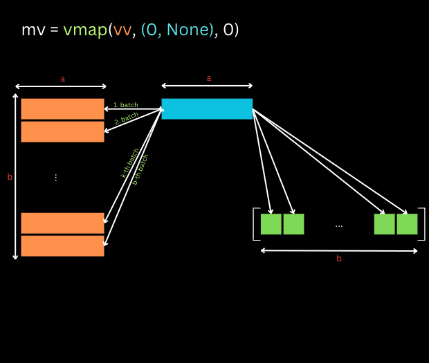
The first function vv defined here leverages JAX’s dot function to perform a vector-vector multiplication, resulting in a scalar. In the code, this is represented as [], depicting that the output is a scalar quantity. The second function conducts matrix-vector multiplication. It accepts a matrix of shape [b, a] and a vector of shape [a], subsequently producing a vector of shape [b]. This function is an extension of the vv function, transformed using vmap with in_axes=[0, None]. In the in_axes parameter, the presence of None specifies to vmap that the corresponding argument (the one in the position of None) should not have a batch dimension introduced. Instead, it indicates that this argument should be treated as it is, without any batch axis, implying it stays consistent across all batched calculations.
The last defined function, mm, is designed to escalate matrix-vector multiplication to matrix-matrix multiplication. This function utilizes mv, which is wrapped with vmap along with the argument in_axes=[None, 1].

In in_axes=[None, 1], the None tells vmap that the first argument should not be treated as a batch, and should remain unchanged across all batch computations. The second argument, represented by the 1, specifies that batching should be carried out across the second axis of this argument. Hence, mm allows for matrix-matrix multiplication, by treating each column of the second matrix as a separate batch for the matrix-vector multiplication.
In the earlier examples, the second argument for the vmap function, known as out_axes, has been omitted. The out_axes parameter is responsible for determining how the results of batch computations are stored across the axes. This means it dictates how the output batch dimension is arranged in the result. By manipulating out_axes, you have control over the placement of the batch dimension in the output. The interpretation of the out_axes argument in vmap mirrors that of the in_axes argument, heavily relying on the specific structure and semantics of your data. Essentially, the meaning of each axis is primarily influenced by the way you’ve arranged your data within the tensor, rather than being inherent to the tensor or the axes themselves.
At the end of this post lets check what performance gain we can achieve by using vmap and making the function to support batching operations with inputs provided to the function.
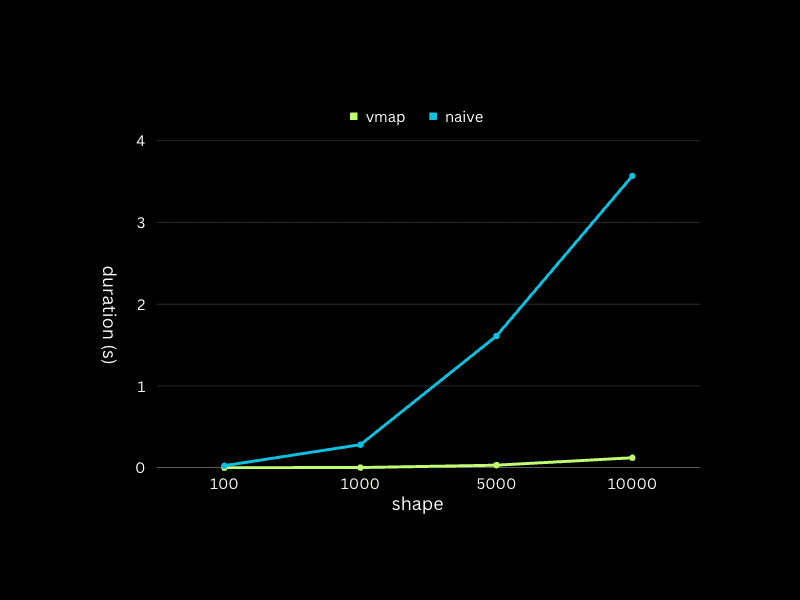
We tested both the vmap method and the naive method with vectors from the same distribution. The test shapes were 100, 1000, 5000, and 10000, meaning we processed a matrix of [shape, shape] for each test.
rnd_key_1 = random.PRNGKey(0)
rnd_key_2 = random.PRNGKey(41)

suggested_shapes = [100, 1_000, 5_000, 10_000]
for shape in suggested_shapes:
    x_batched_random = random.normal(key=rnd_key_1, shape=(shape, ))
    y_batched_random = random.normal(key=rnd_key_2, shape=(shape, ))

    t_result = %timeit -n 100 batched_custom_dot(x_batched_random, y_batched_random).block_until_ready()
The performance chart clearly demonstrates a notable divergence in execution times between the vmap method and the naive method when the shape exceeds 1000. Despite the growing shape of the input vectors, the vmap method consistently keeps the execution time under one second. On the other hand, the execution time for the naive method escalates directly in line with the input vector shape. I conducted the tests on my personal MacBook Pro, which boasts a 2.4 GHz 8-Core Intel Core i9 CPU and 32GB of 2400 MHz DDR4 RAM. Feel free to try the provided code yourself, and experience the efficiency of the vmap method firsthand. Your personal experimentation will only enhance your understanding and appreciation of this powerful tool.
Indeed, our journey through the realm of JAX’s vmap function has come to an end. We’ve seen its ability to handle batched operations with remarkable efficiency, outperforming the naive approach even as the scale of data increases. The role of in_axes and out_axes in structuring computations also came to light, adding a layer of flexibility to our toolkit.
Note that the animations and flow diagrams I present here don’t aim to illustrate the internal workings of the vmap function. Rather, their purpose is to assist in comprehending the high-level concepts, aiding you in effectively utilizing vmap in a variety of different scenarios. They provide a visual guide to understanding how vmap handles data, ultimately supporting you in applying this powerful tool in practice.
As we conclude, remember the power of vmap isn’t merely about execution, but about fostering efficient and scalable computations. And as Master Yoda would put it, “Do. Or do not. There is no try.”
